Simple hyperparameter and architecture search in tensorflow with ray tune
In a previous blog post I have shown a very clean method on how to implement efficient hyperparameter search in tensorflow from scratch. I presented population-based training, an evolutionary method that allows cheap and adaptive hyperparameter search by changing hyperparameters already during training instead of having to train until convergence before the resulting performance statistics can be used to inform the choice of hyperparameters. That said, the vanilla version I presented had two major downsides: The training was not distributed out of the box and also required that the graph is constructed in the beginning and can be reused for different parameter settings.
In this blog post we want to look at the distributed computation framework ray and its little brother ray tune that allow distributed and easy to implement hyperparameter search. It not only supports population-based training but also other hyperparameter search algorithms. Ray and ray tune support any autograd package, including tensorflow and PyTorch.
Setting up ray
Install ray on all your machines
pip install ray
If you only have a single machine at your disposal (it will make use of all local CPU and GPU resources), initialize ray with
import ray

ray.init()
Otherwise, pick a machine to be the head node
ray start --head --redis-port=6379
and connect your other instances
ray start --redis-address=HEAD_HOSTNAME:6379
Finally, run your code on any node
import ray

ray.init(redis_address='HEAD_HOSTNAME:6379')
Having done that, we are ready to distribute tasks such as hyperparameter tuning. More information on how to set up a cluster can be found here.
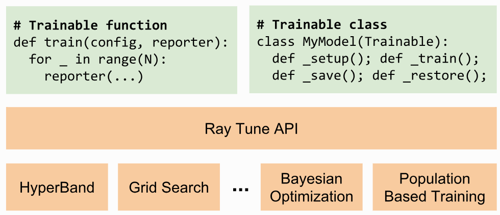
Implementing your model
We will need to implement a model using the following skeleton. You should be able to plug in your existing tensorflow code easily:
import ray.tune as tune

class Model:
  # TODO implement

class MyTrainable(Trainable):
  def _setup(self):
    # Load your data
    self.data = ...
    # Setup your tensorflow model
    # Hyperparameters for this trial can be accessed in dictionary self.config
    self.model = Model(self.data, hyperparameters=self.config)
    # To save and restore your model
    self.saver = tf.train.Saver()
    # Start a tensorflow session
    self.sess = tf.Session()

  def _train(self):
    # Run your training op for n iterations
    for _ in range(n):
      self.sess.run(self.model.training_op)

    # Report a performance metric to be used in your hyperparameter search
    validation_loss = self.sess.run(self.model.validation_loss)
    return tune.TrainingResult(timesteps_this_iter=n, mean_loss=validation_loss)

  def _stop(self):
    self.sess.close()

  # This function will be called if a population member
  # is good enough to be exploited
  def _save(self, checkpoint_dir):
    path = checkpoint_dir + '/save'
    return self.saver.save(self.sess, path, global_step=self._timesteps_total)

  # Population members that perform very well will be
  # exploited (restored) from their checkpoint
  def _restore(self, checkpoint_path):
    return self.saver.restore(self.sess, checkpoint_path)
A new Trainable will be instantiated and executed on an available GPU in your cluster / on your machine for each trial or population member (each having their own hyperparameters) in your population-based training.
Setting up ray tune
Next, register your trainable and specify your experiments
import numpy as np

tune.register_trainable('MyTrainable', MyTrainable)
train_spec = {
  'run': 'MyTrainable',
  # Specify the number of CPU cores and GPUs each trial requires
  'trial_resources': {'cpu': 1, 'gpu': 1},
  'stop': {'timesteps_total': 20000},
  # All your hyperparameters (variable and static ones)
  'config': {
    'batch_size': 20,
    'units': 100,
    'l1_scale': lambda cfg: return np.random.uniform(1e-3, 1e-5),
    'learning_rate': tune.random_search([1e-3, 1e-4])
    ...
  },
  # Number of trials
  'repeat': 4
}
The entry ‘repeat’ describes the number of trials / population members.
Each trial will sample its ‘config’ from the specification above (i.e. using the predefined values or running the specified function).
The instruction tune.random_search will multiply the number of trials by the number of elements it was given, effectively running a grid search.
Finally, we have to define the kind of hyperparameter tuning we would like to perform and start our experiments. This is how it works for population-based training:
pbt = PopulationBasedTraining(
  time_attr='training_iteration',
  reward_attr='mean_loss',
  perturbation_interval=1,
  hyperparam_mutations={
    'l1_scale': lambda: np.random.uniform(1e-3, 1e-5),
    'learning_rate': [1e-2, 1e-3, 1e-4]
  }
)
tune.run_experiments({'population_based_training': train_spec}, scheduler=pbt)
The above example will save, explore and exploit your population every time after _train has been called on your Trainable.
This is because we set ‘perturbation_interval’ to 1.
Furthermore, both ‘l1_scale’, as well as ‘learning_rate’, will be perturbed or resampled during explore operations according to the scheme specified.
You can even implement your own exploration function, to learn more see here.
Because at every mutation step of the population-based training the entire model is saved to disk and restored (and possibly sent to a different machine), ray tune requires a significantly bigger overhead compared to our vanilla tensorflow version. Therefore you might want to increase pertubation_interval depending on the length of each iteration.
Optional: Network morphisms
On the other hand, if your graph needs to be rebuilt anyways, for instance, to make architectural changes based on hyperparameters, the graph reconstruction makes the process quite easy.
To give you an example, let’s say you want to increase the number of units in a layer.
You then could implement a network morphism that keeps your neural network function \(f\) identical but changes the number of units by padding your weight and bias variables with zeros.
You will have to redefine your _restore function
def _restore(self, checkpoint_path):
  reader = tf.train.NewCheckpointReader(checkpoint_path)
  for var in self.saver._var_list:
    tensor_name = var.name.split(':')[0]
    if not reader.has_tensor(tensor_name):
        continue
    saved_value = reader.get_tensor(tensor_name)
    resized_value = fit_to_shape(saved_value, var.shape.as_list())
    var.load(resized_value, self.sess)
where fit_to_shape is defined as
def fit_to_shape(array, target_shape):
  source_shape = np.array(array.shape)
  target_shape = np.array(target_shape)

  if len(target_shape) != len(source_shape):
    raise ValueError('Axes must match')

  size_diff = target_shape - source_shape

  if np.all(size_diff == 0):
    return array

  if np.any(size_diff > 0):
    paddings = np.zeros((len(target_shape), 2), dtype=np.int32)
    paddings[:, 1] = np.maximum(size_diff, 0)
    array = np.pad(array, paddings, mode='constant')

  if np.any(size_diff < 0):
    slice_desc = [slice(d) for d in target_shape]
    array = array[slice_desc]

  return array
Note that in the case where your number of units is reduced, the above code will not keep the function \(f\) identical! One might, for instance, derive a more intelligent algorithm that removes only the weights and biases that have zero magnitudes. This might be encouraged by l1-regularization.
Waiting for results and visualizing
Finally, lean back and let the magic happen. You will see that ray tune outputs nice statistics along the way
== Status ==
PopulationBasedTraining: 42 checkpoints, 28 perturbs
Resources used: 3/12 CPUs, 3/3 GPUs
Result logdir: /home/louis/ray_results/population_based_training
PAUSED trials:
 - Experiment_0:	PAUSED [pid=20781], 971 s, 1600 ts, -1.64e+03 rew, 0.935 loss, 0.676 acc
RUNNING trials:
 - Experiment_1:	RUNNING [pid=23121], 1162 s, 1350 ts, -1.68e+03 rew, 0.994 loss, 0.665 acc
 - Experiment_2:	RUNNING [pid=18700], 979 s, 1550 ts, -1.63e+03 rew, 0.988 loss, 0.663 acc
 - Experiment_3:	RUNNING [pid=22593], 990 s, 1550 ts, -1.77e+03 rew, 0.959 loss, 0.671 acc
To visualize log data both from ray tune and your own tensorflow summaries use Tensorboard
tensorboard --logdir ~/ray_results/population_based_training
If you want to learn more about ray tune, have a look at the documentation and examples.