Hyperparameter search with population based training in tensorflow
Deep learning researchers often spend a large amount of time tuning their architecture and hyper-parameters. A simple method to reduce this human effort is to perform a grid search, essentially random search, on a given range of possible hyper-parameter values. This method is exponential in the number of hyper-parameters and requires to train the entire neural network until convergence for each hyper-parameter setting.
More advanced work such as reinforcement learning for architecture search and evolutionary approaches allow to not only search in the space of hyper-parameters but also architectures. On the downside, these methods are really expensive and require hundreds of GPUs.
Recently, a very simple method for hyper-parameter search has been proposed by DeepMind [1]. In this article, I will showcase the method with a simple tensorflow example. While this method is only suitable for fixed architectures with variable hyper-parameters, there are methods such as network morphisms [2] that allow to extend this approach to architecture search. The implementation of these network morphisms is a bit more complicated, so I will leave an implementation of network morphisms to a follow-up blog post.
Population based training (PBT)
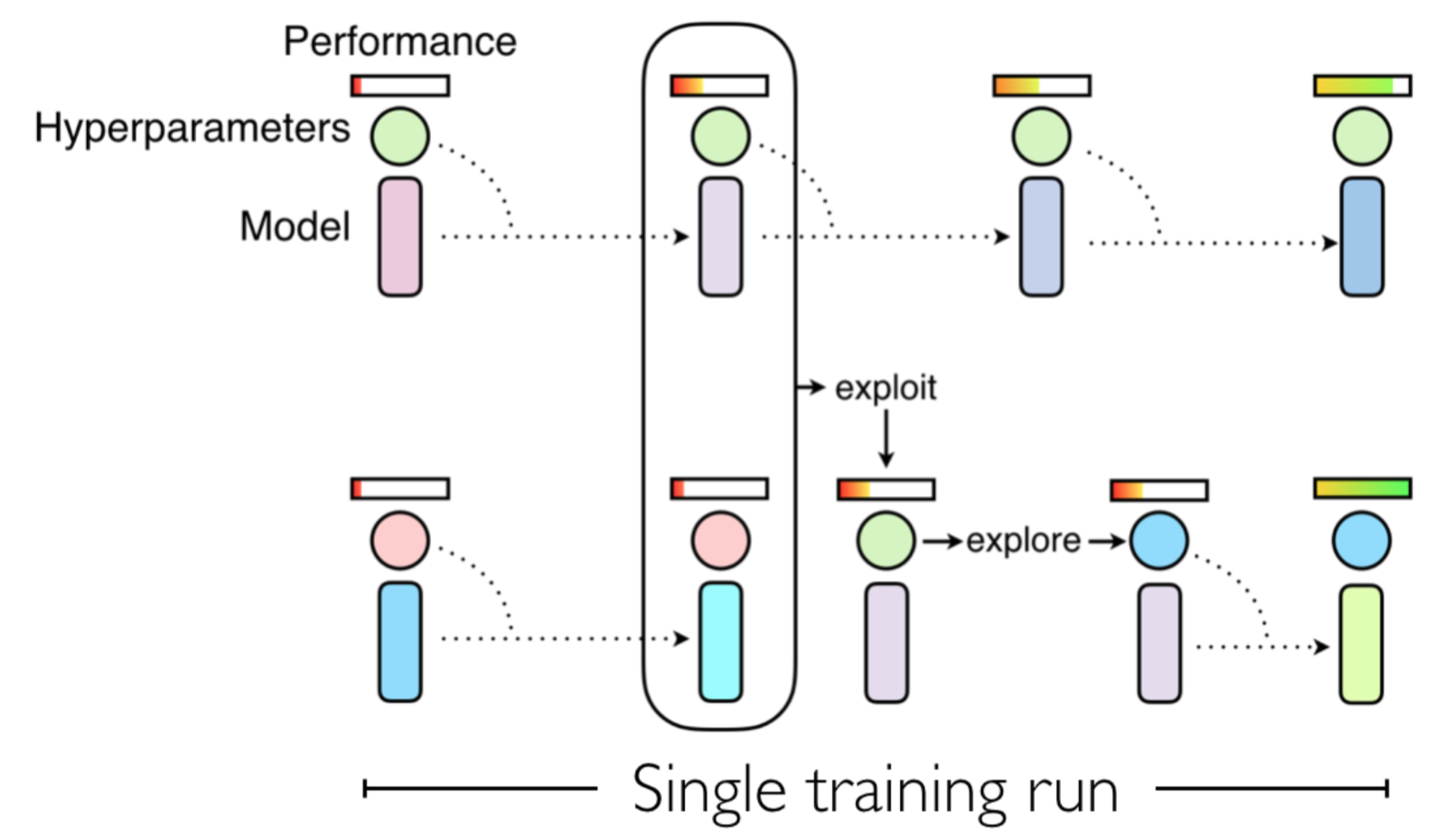
Population based training is based on the idea that we have a population of training runs with different hyper-parameters, and every \(m\) iterations we exploit and explore. Exploitation of the best training runs is defined by overwriting the parameters and hyper-parameters of the worst training runs, while exploration is ensured by perturbation of their hyper-parameters with noise. This procedure is visualized in the following figure.
Implementation in tensorflow
We will do CIFAR10 image classification in this example. Our goal is nothing fancy - just use standard fully connected layers. But how do we choose the capacity for these layers? This is where our population based training comes in - we just specify very large layers and then apply l1-regularization to essentially zero-out unnecessary connections. This prevents overfitting. The scale of this l1-regularizer will be a hyper-parameter and determined by our algorithm.
For this example, we will need tensorflow, numpy, matplotlib and a nice package called ‘observations’ that allows us to load common datasets in seconds.
import tensorflow as tf
import tensorflow.contrib as tfc
import numpy as np
import matplotlib.pyplot as plt
import observations
from functools import lru_cache
These few lines of code are literally everything we need to create two tf.Dataset instances of the CIFAR10 dataset for training and testing.
tf.reset_default_graph()

train_data, test_data = observations.cifar10('data/cifar',)
test_data = test_data[0], test_data[1].astype(np.uint8) # Fix test_data dtype

train = tf.data.Dataset.from_tensor_slices(train_data).repeat().shuffle(10000).batch(64)
test = tf.data.Dataset.from_tensors(test_data).repeat()
We now create an iterator to iterate over either the training or test data. For that, we use iterator handles as described in the tensorflow documentation.
handle = tf.placeholder(tf.string, [])
itr = tf.data.Iterator.from_string_handle(handle, train.output_types, train.output_shapes)
inputs, labels = itr.get_next()

def make_handle(sess, dataset):
  iterator = dataset.make_initializable_iterator()
  handle, _ = sess.run([iterator.string_handle(), iterator.initializer])
  return handle
The two tensors inputs and labels now contain the data, we cast them to the right data types and shape.
inputs = tf.cast(inputs, tf.float32) / 255.0
inputs = tf.layers.flatten(inputs)
labels = tf.cast(labels, tf.int32)
Next, we create the model we’ll be using to classify CIFAR10 images.
class Model:

  def __init__(self, model_id: int, regularize=True):
    self.model_id = model_id
    self.name_scope = tf.get_default_graph().get_name_scope()

    # Regularization
    if regularize:
      l1_reg = self._create_regularizer()
    else:
      l1_reg = None

    # Network and loglikelihood
    logits = self._create_network(l1_reg)
    # We maximixe the loglikelihood of the data as a training objective
    distr = tf.distributions.Categorical(logits)
    loglikelihood = distr.log_prob(labels)

    # Define accuracy of prediction
    prediction = tf.argmax(logits, axis=-1, output_type=tf.int32)
    self.accuracy = tf.reduce_mean(tf.cast(tf.equal(prediction, labels), tf.float32))

    # Loss and optimization
    self.loss = -tf.reduce_mean(loglikelihood)
    # Retrieve all weights and hyper-parameter variables of this model
    trainable = tf.get_collection(tf.GraphKeys.TRAINABLE_VARIABLES, self.name_scope + '/')
    # The loss to optimize is the negative loglikelihood + the l1-regularizer
    reg_loss = self.loss + tf.losses.get_regularization_loss()
    self.optimize = tf.train.AdamOptimizer().minimize(reg_loss, var_list=trainable)

  def _create_network(self, l1_reg):
    # Our deep neural network will have two hidden layers with plenty of units
    hidden = tf.layers.dense(inputs, 1024, activation=tf.nn.relu,
                             kernel_regularizer=l1_reg)
    hidden = tf.layers.dense(hidden, 1024, activation=tf.nn.relu,
                             kernel_regularizer=l1_reg)
    logits = tf.layers.dense(hidden, 10,
                             kernel_regularizer=l1_reg)
    return logits

  def _create_regularizer(self):
    # We will define the l1 regularizer scale in log2 space
    # This allows changing one unit to half or double the effective l1 scale
    self.l1_scale = tf.get_variable('l1_scale', [], tf.float32, trainable=False,
                                    initializer=tf.constant_initializer(np.log2(1e-5)))
    # We define a 'pertub' operation that adds some noise to our regularizer scale
    # We will use this pertubation during exploration in our population based training
    noise = tf.random_normal([], stddev=0.5)
    self.perturb = self.l1_scale.assign_add(noise)

    return tfc.layers.l1_regularizer(2 ** self.l1_scale)

  @lru_cache(maxsize=None)
  def copy_from(self, other_model):
    # This method is used for exploitation. We copy all weights and hyper-parameters
    # from other_model to this model
    my_weights = tf.get_collection(tf.GraphKeys.GLOBAL_VARIABLES, self.name_scope + '/')
    their_weights = tf.get_collection(tf.GraphKeys.GLOBAL_VARIABLES, other_model.name_scope + '/')
    assign_ops = [mine.assign(theirs).op for mine, theirs in zip(my_weights, their_weights)]
    return tf.group(*assign_ops)
We will have to create several models, one for each population member. Each population member will have separate hyper-parameters and weights.
def create_model(*args, **kwargs):
  with tf.variable_scope(None, 'model'):
    return Model(*args, **kwargs)
Now, let’s train a standard neural network without regularization to obtain a baseline we are competing with.
ITERATIONS = 50000

nonreg_accuracy_hist = np.zeros((ITERATIONS // 100,))
model = create_model(0, regularize=False)

with tf.Session() as sess:
  train_handle = make_handle(sess, train)
  test_handle = make_handle(sess, test)
  sess.run(tf.global_variables_initializer())

  feed_dict = {handle: train_handle}
  test_feed_dict = {handle: test_handle}
  for i in range(ITERATIONS):
    # Training
    sess.run(model.optimize, feed_dict)
    # Evaluate
    if i % 100 == 0:
      nonreg_accuracy_hist[i // 100] = sess.run(model.accuracy, test_feed_dict)
The following is essentially the core of population based training. We create a population of models, and repeatedly
- Exploit the best models by discarding the worst models and replacing them with the weights and hyper-parameters of the best model
- Explore the search space of hyper-parameters by adding noise through the
perturboperation - Train each population member for a certain amount of iterations
- Evaluate each population member in terms of their validation set accuracy
NOTE: In this example we actually used the test set for scoring instead of the validation set. In practice, you should not do this because it might lead to overfitting to the test set. In the case of l1-regularization, it is highly unlikely that we can actually overfit in a meaningful way, but it is certainly not best-practice. In principle, you could partition the training set into a training and validation set.
POPULATION_SIZE = 10
BEST_THRES = 3
WORST_THRES = 3
POPULATION_STEPS = 500
ITERATIONS = 100

accuracy_hist = np.zeros((POPULATION_SIZE, POPULATION_STEPS))
l1_scale_hist = np.zeros((POPULATION_SIZE, POPULATION_STEPS))
best_accuracy_hist = np.zeros((POPULATION_STEPS,))
best_l1_scale_hist = np.zeros((POPULATION_STEPS,))

models = [create_model(i) for i in range(POPULATION_SIZE)]

with tf.Session() as sess:
  train_handle = make_handle(sess, train)
  test_handle = make_handle(sess, test)
  sess.run(tf.global_variables_initializer())

  feed_dict = {handle: train_handle}
  test_feed_dict = {handle: test_handle}
  for i in range(POPULATION_STEPS):
    # Copy best
    sess.run([m.copy_from(models[0]) for m in models[-WORST_THRES:]])
    # Perturb others
    sess.run([m.perturb for m in models[BEST_THRES:]])
    # Training
    for _ in range(ITERATIONS):
      sess.run([m.optimize for m in models], feed_dict)
    # Evaluate
    l1_scales = sess.run({m: m.l1_scale for m in models})
    accuracies = sess.run({m: m.accuracy for m in models}, test_feed_dict)
    models.sort(key=lambda m: accuracies[m], reverse=True)
    # Logging
    best_accuracy_hist[i] = accuracies[models[0]]
    best_l1_scale_hist[i] = l1_scales[models[0]]
    for m in models:
      l1_scale_hist[m.model_id, i] = l1_scales[m]
      accuracy_hist[m.model_id, i] = accuracies[m]
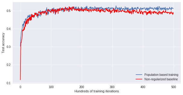
Let’s see how well we are doing. In the following graph we compare our baseline with the best model throughout our population based training. Clearly, our method overfits less than the baseline, achieving higher test accuracies at the end of training.
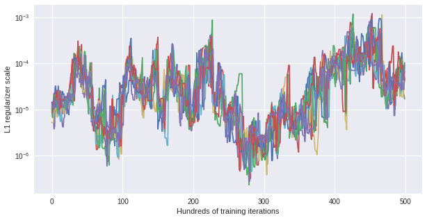
Another interesting observation can be made looking at the changing l1 scale for each of the models. Instead of fluctuating around the initial value \(10^{-5}\) there is an evolving pattern over time. This means, depending on the time in training, different l1 regularization is optimal to gain maximal test accuracy.
All code can be found in this github gist.
Closing remarks
Obviously, we could have done much better by using convolutions on CIFAR10 image classification. But nevertheless, the concept of population based training can be applied to any machine learning problem involving hyper-parameters: supervised, unsupervised and reinforcement learning. If you have an interesting application, leave it in the comments!
Also, we’ve been training all population members on the same GPU, waiting for all of them to finish before exploring and exploiting. In a larger setup, we will want to train each member on a separate GPU asynchronously. This can be extended to a distributed setup with multiple machines, which I may explore in another blog post. I’ve also mentioned architecture search and network morphisms already – that’s when all this stuff gets really exciting!