Theories of Intelligence (1/2): Universal AI
Many AI researchers, in particular in the field of deep learning and reinforcement learning, pursue a bottom-up approach. We reason by analogy to neuroscience and aim to solve current limitations of AI systems on a case-by-case basis. While this allows for steady progress, it is unclear which properties of an artificial intelligence system are required to be engineered and which may be learned. In fact, one might argue that any design decision by a human can be outperformed by a learned rule, given enough data. The less data we have, the more inductive biases we have to build into our systems. But how do we know which aspects of an artificial system are necessary and which are better left to learn? I want to give insight into a theoretic top-down approach of universal artificial intelligence. It promises to prove what an optimal agent for any set of environments would have to look like and how intelligence can be measured. Furthermore, we will learn about theoretical limits of (non-)computable intelligence.
The post is structured as follows
- We try to define intelligence
- We motivate how Epicurus’ principle and Occam’s razor relate to the problem of intelligence
- We introduce optimal sequence prediction using Solomonoff induction
- We extend our agent to active environments (Reinforcement Learning paradigm) and show its optimality
- We define a formal measure of intelligence
This blog post is, in most parts, based on Marcus Hutter’s book Universal Artificial Intelligence and Shane Legg’s PhD thesis Universal Super Intelligence.
- Most machine learning tasks can be reduced to sequence prediction in passive or active environments
- Sequences, environments, and hypotheses have universal prior probabilities based on Epicurus’ principle and Occam’s razor
- The central quantity is the Kolmogorov complexity, a measure of complexity
- Using these prior probabilities we can construct universally optimal sequence prediction and agents in active environments
- The intelligence of an agent can be formally defined to be its performance in all environments weighted by complexity
- We can derive the universal agent AIXI that maximizes this intelligence measure
- Any other agent that is better than AIXI in a specific environment will be at least as much worse in some other environment
What is intelligence?
What is intelligence? While there are many colloquial meanings of intelligence, many intelligence tests have been developed that can predict future academic or commercial performance very well. But these tests are limited in scope because they only work for humans and might even be prone to cultural biases. Additionally, how do we compare the intelligence of animals or machines with humans? It seems that intelligence is not as easy to define as one might think. If our goal is to design the most intelligent agent, we better define the term as precisely and general as possible.
Among many definitions of intelligence one can extract two very common aspects: Firstly, intelligence is seen as a property of an actor interacting with an external environment. Secondly, intelligence is related to this actor’s ability to succeed, implying the existence of some kind of goal. It is therefore fair to say that the greater the capability of an actor to reach certain goals in an environment, the greater the individual’s intelligence. It is also noteworthy that when describing intelligence, the focus is often on adaptation, learning, and experience. Shane Legg argues that this is an indicator that the true environment in which these goals are pursued is not fully known and needs to be discovered first. The actor, therefore, needs to quickly learn and adapt in order to perform as well as possible in a wide range of environments. This leads us to a simple working definition that intuitively covers all aspects of intelligence:
Intelligence measures an agent’s ability to achieve goals in a wide range of environments.
Universal Artificial Intelligence
In the following, we will derive the universal artificial intelligence AIXI. It will be based on three fundamental principles: Epicurus’ principle of multiple explanations, Occam’s razor, and Bayes’ rule. While Epicurus’ principle and Occam’s razor are important to motivate AIXI, none of the proofs rely on them as assumptions.
All intelligent agents will have to make predictions to achieve their goals. Only if the underlying generating process can (approximately) be modeled by such an agent it can determine whether progress toward the goal is being made. In this context, we model hypotheses \(h \in \mathcal{H}\) of the generating process that explain the data. This may be the dynamics of an environment or the probability distribution over a sequence. Epicurus’ principle of multiple explanations states
Keep all hypotheses that are consistent with the data.
Intuitively, this makes sense because future evidence may increase the likelihood of any current hypothesis. This also implies that we will have to store the entire previous sequence or interaction history. Any information that is discarded may be informative in the future. Bayes’ rule defines how we need to integrate our observations \(D\) to yield a posterior probability \(P(h|D)\)
\[P(h|D) = \frac{P(D|h)P(h)}{P(D)}\]While we can find \(P(D)\) by marginalization, we are faced with a problem: Where does the prior \(P(h)\) come from? Bayesian statisticians argue that domain knowledge can be used to inform the prior \(P(h)\). In the absence of such knowledge, one can simply impose a uniform prior (indifference principle). This works great for finite sets \(\mathcal{H}\) but leads to problems with non-finite hypothesis spaces where the use of an improper prior is required. In addition, the uniform prior highly depends on the problem formulation and is not invariant to reparameterization and group transformations. A simple example illustrates that: We could have three hypotheses \(\mathcal{H}_3 := \{\text{heads biased}, \text{tails biased}, \text{fair}\}\) for a coin flip. Alternatively, we can regroup our hypotheses to \(\mathcal{H}_2 := \{\text{biased}, \text{fair}\}\). Depending on the grouping chosen, the uniform prior will assign a different probability to the hypothesis \(h_b = \text{biased}\). Occam’s razor will solve this issue. It roughly says
Among all hypotheses that are consistent with the observations, the simplest is most likely.
Occam’s razor can be motivated from several perspectives. Empirically, hypotheses that make fewer assumptions are more testable and have led to theories that capture the underlying structure better and thus have better predictive performance. Any human not adhering to this principle would be judged irrational. In probability theory, by definition, all assumptions introduce possibilities of error. If an assumption does not improve the accuracy of a theory, its only effect is to increase the probability that the overall theory is wrong.
There is one additional important observation before we can make use of Occam’s razor: While we could define a prior on hypotheses \(P(h)\) as previously shown, there is an equivalent formulation where we use a prior for sequences \(P(x)\). Let’s consider our data \(D\) to be a (binary) sequence \(x \in \mathbb{B}^*\). Bayesian probability theory requires predictions over sequence continuations \(x_{t+1}\) given \(x_{1:t}\) to be weighted, i.e.
\[P(x_{t+1}|x_{1:t}) = \sum_{h \in \mathcal{H}} P(h|x_{1:t}) P(x_{t+1}|x_{1:t}, h)\]where \(P(h|x_{1:t})\) is the posterior defined by Bayes’ rule, therefore requiring a prior \(P(h)\). We can rewrite
\[\begin{align} P(x_{t+1}|x_{1:t}) &= \sum_{h \in \mathcal{H}} P(h|x_{1:t}) P(x_{t+1}|x_{1:t}, h) \\ &= \sum_{h \in \mathcal{H}} \frac{P(x_{1:t}|h)P(h)}{P(x_{1:t})} \frac{P(x_{1:t+1}|h)}{P(x_{1:t}|h)} \\ &= \frac{P(x_{1:t+1})}{P(x_{1:t})} \end{align}\]such as that we now require a prior over sequences. Such a prior over sequences \(x \in \mathbb{B}^*\) is what we will have to find.
So far, we have shown the relevance of finding the right prior probability distribution which may either be expressed over hypothesis space or sequence space. Furthermore, we motivated why Epicurus’ principle of multiple explanations and Occams’ razor may help us to solve this issue.
Solomonoff’s prior and Kolmogorov complexity
Next, in order to solve our problem with prior probabilities, we will formalize a so-called universal prior probability for sequences, hypotheses, and environments based on Epicurus’ principle of multiple explanations and Occam’s razor. We begin with the simplest case, directly defining a prior over sequences.
Let’s extend the sequence prediction problem we briefly introduced. Let \(\mu\) be the true generating distribution over an infinite sequence \(\omega \in \mathbb{B}^{\infty}\). Sequence prediction is a quite powerful framework because any supervised prediction problem can be reduced to such sequence prediction. The task of predicting \(\omega_{t+1}\) after having seen \(\omega_{1:t}\) is known as induction.
Occam’s razor is formalized by Solomonoff’s prior probability for (binary) sequences. Intuitively, a sequence \(x \in \mathbb{B}^*\) is more likely if it is generated by many and short programs \(p\) fed to a universal Turing Machine \(U\). You can think of the program \(p\) as a description of the sequence \(x\). And the Turing Machine \(U\) executes your program \(p\) to generate \(x\). If you can describe \(x\) with few instructions (say bits \(l(p)\)) it must be simpler, and therefore more likely. We describe this probability thus simply with \(2^{-l(p)}\). Also, if there are many explanations for \(x\), we just sum these probabilities.
We can now formally put these intuitions together: We say Turing Machine \(U\) generates \(x\) if \(x\) is a prefix of the output of \(U(p)\). For this prefix with any continuation, we write \(x*\). Solomonoff’s prior probability that a sequence begins with binary string \(x \in \mathbb{B}^*\) is given by
\[M(x) := \sum_{p:U(p)=x*} 2^{-l(p)}\]where \(l(p)\) is the length of program \(p\) and \(U\) is a prefix universal Turing Machine. The fact that we use a prefix universal Turing Machine is a technicality. Such a Turing Machine ensures that no valid program for \(U\) is a prefix of any other. In this definition \(2^{-l(p)}\) can be interpreted as the probability that program \(p\) is sampled uniformly from all possible programs, halving the probability for each additional bit.
To summarize, Solomonoff’s prior probability assigns sequences generated by shorter programs higher probability. We say sequences generated by shorter programs are less complex.
We can further formalize the complexity of a sequence. Instead of taking into account all possible programs \(p\) that could generate a sequence \(x\) we just report the shortest program. Formally, the Kolmogorov complexity of an infinite sequence \(\omega \in \mathbb{B}^\infty\) is the length of the shortest program that produces \(\omega\), given by
\[K(\omega) := \min_{p \in \mathbb{B}^*}\{l(p): U(p) = \omega\}\]Similarly, the Kolmogorov complexity over finite strings \(x \in \mathbb{B}^*\) is the length of the shortest program that outputs \(x\) and then halts.
We have seen how to formalize Occams’ razor to derive a prior probability distribution. In principle, we could now directly apply Solomonoff’s universal prior probability \(M(x)\) to perform induction. But it will be useful to define an alternative variant that takes our hypotheses into account.
Solomonoff-Levin prior
Another way to look at the problem is to define a universal prior probability over hypotheses. It will allow us to define an alternative prior over sequences known as the Solomonoff-Levin prior probability.
We start by defining our hypothesis space \(M_e\) over possible distributions and assume that the true generating distribution \(\mu \in M_e\).
\[M_e := v_1, v_2, v_3, \ldots\]Each \(v_i \in M_e\) is a so-called enumerable probability semi-measure. For now, it is sufficient to know that such a measure assigns each prefix sequence \(x \in \mathbb{B}^*\) of \(\omega\) a probability. Therefore, with such a measure we can describe a distribution over sequences. In order to make sure that \(\mu \in M_e\) we will pick a really large set of hypotheses. In technical terms, \(M_e\) is a computable enumeration of enumerable probability semi-measures. If you are interested in the mathematical details, refer to the optional section.
The index \(i\) can be used a representation of the semi-measure. To assign hypothesis \(v_i\) a probability, we can make use of the Kolmogorov complexity again! If we can describe \(i\) with a short program \(p\), \(v_i\) must be simple. Formally, we define the Kolmogorov complexity for each of the \(v_i \in M_e\) as
\[K(v_i) := \min_{p \in \mathbb{B}^*} \{ l(p): U(p) = i \}\]where \(v_i\) is the \(i^{th}\) element in our enumeration.
This gives us all the tools to define a prior probability for hypotheses! We just assign simpler hypotheses larger probabilities, prescribed by the Kolmogorov complexity from above. Each hypothesis \(v \in M_e\) is assigned a universal algorithmic prior probability
\[P_{M_e}(v) := 2^{-K(v)}\]Finally, we construct a mixture to define a prior over the space of sequences, arriving at the Solomonoff-Levin prior probability of a binary sequence beginning with string \(x \in \mathbb{B}^*\)
\[\xi(x) := \sum_{v \in M_e} P_{M_e}(v) v(x)\]
In order to derive AIXI we will require three concepts that may not be familiar to the reader: Probability (semi-)measures, enumerable functions, and computable enumerations. We denote a sequence \(xy\) as the concatenation of \(x \in \mathbb{B}^*\) and \(y \in \mathbb{B}^*\).
A probability measure is a function over binary sequences \(v: \mathbb{B}^* \to [0, 1]\) such that
\[v(\epsilon) = 1, \forall x \in \mathbb{B}^*: v(x) = v(x0) + v(x1)\]where \(\epsilon\) is the empty string. In other words, we assign each finite binary sequence \(x \in \mathbb{B}^*\) (which could be a prefix of \(\omega\)) a probability such that they consistently add up.
A generalization is the probability semi-measure
\[v(\epsilon) \leq 1, \forall x \in \mathbb{B}^*: v(x) \geq v(x0) + v(x1)\]that can be normalized to a probability measure.
Intuitively, a function is enumerable if it can be progressively approximated from below with a Turing machine in finite time. Conversely, a function is co-enumerable if it can be progressively approximated from above with a Turing machine in finite time.
We stated that we’d like to enumerate enumerable semi-measures. Note that an enumeration is different from an enumerable function. What is a computable enumeration? Basically, we want to enumerate all semi-measures with a Turing Machine in a computable manner. We can not directly output probability measures using our Turing Machine and therefore use its index \(i\) as a description that can then be used to approximate \(v_i(x)\) from below. More precisely, there exists a Turing Machine \(T\) that for any enumerable semi-measure \(v \in M_e\) there exists an index \(i \in \mathbb{N}\) such that
\[\forall x \in \mathbb{B}^*: v(x) = v_i(x) := \lim_{k \to \infty}T(i, k, x)\]with \(T\) increasing in \(k\). In other words, we have a Turing Machine \(T\) and for a given sequence \(x\) and index \(i\) we approximate the value of the semi-measure \(v_i\) for \(x\) from below. The argument \(k\) intuitively describes how exact this approximation shall be. In the limit of \(\lim_{k \to \infty}\) we will yield the exact value \(v_i(x)\).
Why can the index \(i\) be used to define the Kolmogorov complexity for each hypothesis \(v_i \in M_e\)? The more complex \(i\) is, the more complex is the input to the above Turing machine \(T\). For a given \(k\) and \(x\) the complexity of the output can therefore only depend on \(i\).
Solomonoff induction
We now have two formulations for prior distributions over binary sequences: The Solomonoff prior \(M\) and the Solomonoff-Levin prior \(\xi\). Both priors can be shown to only be a multiplicative constant away from each other, i.e. \(M \overset{\times}{=} \xi\). We will need the second formulation \(\xi\) to construct our universal agent AIXI. But for now, let’s focus on the sequence prediction problem.
By the definition of conditional probability our prediction problem reduces to
\[\xi(\omega_{t+1}|\omega_{1:t}) = \frac{\xi(\omega_{1:t+1})}{\xi(\omega_{1:t})}\]Because we used \(\xi\) as our universal prior, this is known as Solomonoff induction for sequence prediction.
Hooray, we’ve done it! But what do we gain from all this? Given this scheme of induction, how good is the predictor \(\xi(\omega_{t+1}|\omega_{1:t})\) relative to the true \(\mu(\omega_{t+1}|\omega_{1:t})\)? It turns out that as long as \(\mu\) can be described by a computable distribution (which is a very minor restriction) our estimator \(\xi\) will converge rapidly to the true \(\mu\), in effect solving the problem optimally!
Convergence of Solomonoff induction
optional sectionWe can measure the relative performance of \(\xi\) to \(\mu\) using the prediction error \(S_t\) given by
\[S_t = \sum_{x \in \mathbb{B}^{t-1}} \mu(x)(\xi(x_t = 0|x) - \mu(x_t = 0|x))^2\]Consider the set of computable probability measures \(M_c \subset M_e\). It can be shown that for any \(\mu \in M_c\) the sum of all prediction errors is bounded by a constant
\[\sum_{t=1}^{\infty} S_t \leq \frac{\ln 2}{2} K(\mu)\]Due to this bound, it follows that the estimator \(\xi\) rapidly converges for any \(\mu\) that can be described by a computable distribution (see Hutter 2007 for what ‘rapid’ describes).
Active environments
So far we only dealt with passive environments in the form of sequence predictions. We will now extend the framework to active environments using the Reinforcement Learning framework as depicted below.

We define an environment to be the tuple \((A, O, R, \mu)\):
- \(A\) is the of all actions our agent can take
- \(O\) is the set of observations the agent can receive
- \(R\) is the set of possible rewards
- \(\mu\) is the environment’s transition probability measure (as defined in the following)
We express the concatenation of observation and reward as \(x := or\). The index \(t\) of a sequence \(ax_t\) refers to both action \(a\) and input \(x\) at time \(t\). Then \(\mu\) is simply the probability measure over transitions \(\mu(x_t|ax_{<t}a_t)\). Depending on the design objective of the agent we will have to specify two signals to yield a well-defined optimally informed agent. Firstly, a communication stream of rewards needs to be specified. This could be something like pain or reward signals similar to what humans experience. Secondly, we need to specify a temporal preference. This can be done in two ways. We may specify a discount factor \(\gamma_t\) directly, for instance, a geometrically decreasing discount factor as commonly seen in the RL-literature:
\[\forall i: \gamma_i := \alpha^i \qquad \text{for} \quad \alpha \in (0, 1)\]Alternatively, we require that the total reward is bounded, therefore directly specifying our preferences in the stream of rewards. We call this set of environments reward-summable environments \(\mathbb{E} \subset E\).
It is a known result that the optimal agent in environment \(\mu\) with discounting \(\gamma\) would then be defined using the Bellman equation
\[\pi^\mu := \arg\max_\pi V_\gamma^{\pi\mu} \\ V_\gamma^{\pi\mu}(ax_{<t}) = \sum_{ax_t} [\gamma_t r_t + V_\gamma^{\pi\mu}(ax_{1:t})]\overset{\pi}{\mu}(ax_t|ax_{<t}) \\\]where \(\overset{\pi}{\mu}\) is the probability distribution jointly over policy and environment, e.g.
\[\overset{\pi}{\mu}(ax_{1:2}) := \pi(a_1) \mu(x_1|a_1) \pi(a_2|ax_1) \mu(x_2|ax_1a_2)\]If the environment \(\mu\) was known we could directly infer the optimal action \(a_t^{\pi^\mu}\) in the \(t^{th}\) step
\[a_t^{\pi^\mu} := \arg\max_{a_t} \lim_{m \to \infty} \sum_{x_t} \max_{a_{t+1}} \sum_{x_{t+1}} \ldots \max_{a_m} \sum_{x_m} [\gamma_t r_t + \ldots + \gamma_m r_m] \mu(x_{t:m}|ax_{<t}a_{t:m})\]But it is easy to see that this agent does not fulfill our intelligence definition yet. The agent needs to be able to cope with many different environments and learn from them, therefore it can not have \(\mu\) precoded. We will take the agent from above and replace the environment dynamics \(\mu\) with the generalized universal prior distribution \(\xi\).
Again, we will have hypotheses, this time over possible environment probability measures. Formally, our environment hypothesis space will now be the set of all enumerable chronological semi-measures
\[E := \{v_1, v_2, \ldots\}\]We call these measures chronological because our sequence of interactions with the environment has a time component. Again, we define the universal prior probability of a chronological environment \(v \in E\) using the Kolmogorov complexity
\[P_E(v) := 2^{-K(v)}\]where \(K(v)\) is the length of the shortest program that computes the environment’s index. We yield the prior over the agent’s observations by constructing another mixture
\[\xi(x_{1:n}|a_{1:n}) := \sum_{v\in E} 2^{-K(v)} v(x_{1:n}|a_{1:n})\]By replacing \(\mu\) with \(\xi\) (and using conditional probability) we finally yield the universal AIXI agent \(\pi^\xi\):
Convergence
Can we show that \(\xi\) converges to the true environment \(\mu\) in the same way we have shown that our universal prior \(\xi\) for sequence prediction converged? Indeed, we can, but with a strong limitation: The interaction history \(ax_{<t}\) must come from \(\pi^\mu\). Of course, \(\mu\) is unknown and this is not feasible. Even worse, it can be shown that it is in general impossible to match the performance of \(\pi^\mu\). Different from the sequence prediction problem, possibly irreversible interaction with the environment is necessary. To give a very simple example: Let’s imagine an environment where an agent has to pick between two doors. One door leads to hell (very little reward), the other to heaven (plenty of reward). Crucially, after having chosen one door, the agent can not return. But because the agent does not have any prior knowledge about what is behind the doors, there is no optimal behavior that guarantees that heaven is chosen. Conversely, if \(\mu\) was known to the agent, it could infer which door leads to larger rewards. We will investigate this problem again in a later section. For now, let’s at least investigate whether we are as optimal as any agent can be in such a situation.
Luckily, there is a key theorem proven by Hutter that says exactly that. Let \(\pi^\zeta\) be the equivalent of agent \(\pi^\xi\) defined over \(\mathcal{E} \subseteq E\) instead of \(E\), then we have
For any \(\mathcal{E} \subseteq E\) the agent \(\pi^\zeta\) is Pareto optimal.
An agent \(\pi\) is Pareto optimal if there is no other agent \(\rho\) such that
\[\forall \mu \in \mathcal{E} \quad \forall ax_{<t}: V_\gamma^{\rho\mu}(ax_{<t}) \geq V_\gamma^{\pi\mu}(ax_{<t})\]with strict inequality for at least one \(\mu\).
In other words, there exists no agent that is at least as good as \(\pi^\zeta\) in all environments in \(\mathcal{E}\), and strictly better in at least one. An even stronger result can be shown: \(\pi^\zeta\) is also balanced Pareto optimal which means that any increase in performance in some environment due to switching to another agent is compensated for by an equal or greater decrease in performance in some other environment.
Great! But even if we can not construct a better agent, for what kind of environments is our agent \(\pi^\xi\) guaranteed to converge to the optimal performance of \(\pi^\mu\)? Intuitively, the agent needs to be given time to learn about its environment \(\mu\) to reach optimal performance. But due to irreversible interaction, not all environments permit this kind of behavior. We formalize this concept of convergence by defining self-optimizing agents and categorizing environments into the ones admitting self-optimizing agents, and the ones that do not. An agent \(\pi\) is self-optimizing in an environment \(\mu\) if,
\[\frac{1}{\Gamma_t}V_\gamma^{\pi\mu}(ax_{<t}) \to \frac{1}{\Gamma_t} V_{\gamma}^{\pi^\mu\mu}(\hat a \hat x_{<t}) \qquad \text{where} \quad \Gamma_t := \sum_{i=t}^{\infty} \gamma_i\]with probability 1 as \(t \to \infty\). The interaction histories \(ax_{<t}\) and \(\hat a \hat x_{<t}\) are sample from \(\pi\) and \(\pi^\mu\) respectively. We require normalization \(\frac{1}{\Gamma_t}\) because un-normalized expected future discounted reward always converges to zero. Intuitively, the above statement says that with high probability the performance of a self-optimizing agent \(\pi\) converges to the performance of the optimal agent \(\pi^\mu\). Furthermore, it can be proven that if there exists a sequence (agent might be non-stationary) of self-optimizing agents \(\pi_m\) for a class of environments \(\mathcal{E}\), then the agents \(\pi^\zeta\) is also self-optimizing for \(\mathcal{E}\) [proof in Hutter 2005]. This is a promising result because while not all environments admit self-optimizing agents we can rest assured that the ones who do will result in \(\pi^\zeta\) being self-optimizing.
For the commonly used Markov Decision Process (MDP) it can be shown that if it is ergodic, then it admits self-optimizing agents. We say that an MDP environment \((A, X, \mu)\) is ergodic iff there exists an agent \((A, X, \pi)\) such that \(\overset{\pi}{\mu}\) defines an ergodic Markov chain. Other self-optimizing environments are summarized in the following figure.
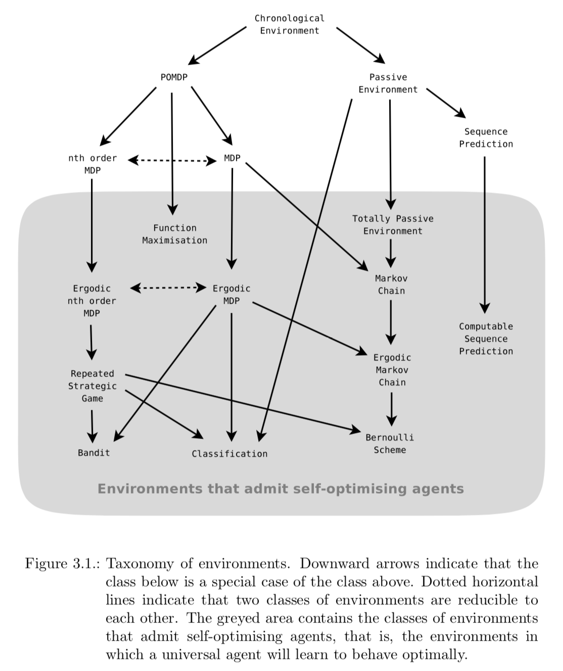
It is important to note, that being self-optimizing only tells us about the performance in the limit, not how quickly the agent will learn to perform well. While we were able to upper-bound the error by a constant in the case of sequence prediction, such a general result is impossible for active environments. Further research is required to prove convergence results for different classes of environments. Due to the Pareto optimality of AIXI, we can at least be confident that no other agent could converge more quickly in all environments.
What about exploration?
You may wonder why the RL exploration problem does not appear in our universal agent. The answer is that exploration is optimally encoded in our universal prior \(\xi\). All possible environments are being considered, weighted by their complexity, such that actions are considered not just with respect to the optimal policy in a single environment, but all environments.
Measuring intelligence
Up until now, we derived the universal agent AIXI based on our working definition of intelligence.
Intelligence measures an agent’s ability to achieve goals in a wide range of environments.
In the following, we reverse the process and aim to define intelligence itself mathematically such that it permits us to measure intelligence universally for humans, animals, machines or any other arbitrary forms of intelligence. This may even allow us to directly optimize for the intelligence of our agents instead of surrogates such as spreading genes, survival or any other objective we specify as designers.
We have already derived a pretty powerful toolbox to define such a formal measure of intelligence. We formalize the wide range of environments and any goal that could be defined in these with the class of reward-summable environments \(\mathbb{E}\). The ability of the agent \(\pi\) to achieve these goals is then just its value function \(V_\mu^\pi\). We arrive at the following very simple formulation:
The universal intelligence of an agent \(\pi\) is its expected performance with respect to the universal distribution \(2^{-K(\mu)}\) over the space of all computable reward-summable environments \(\mathbb{E} \subset E\), that is,
\[\Upsilon(\pi) := \sum_{\mu \in \mathbb{E}} 2^{-K(\mu)} V_\mu^\pi\]This very simple measure of intelligence is remarkably close to our working definition of intelligence! All we have added to our informal definition is a preference over environments we care about in the form of the prior probability \(2^{-K(\mu)}\).
How does this measure relate to AIXI? By the linearity of expectation the above definition is just the expected future discounted return \(V_\xi^\pi\) under the universal prior probability distribution \(\xi\):
\[\begin{align} V_\xi^\pi &= V_\xi^\pi(\epsilon) \\ &= \sum_{ax_1}[r_t + V_\xi^\pi(ax_1)]\xi(x_1)\pi(a_1|x_1) \\ &= \sum_{ax_1}[r_t + V_\xi^\pi(ax_1)]\sum_{\mu \in \mathbb{E}} 2^{-K(\mu)} \mu(x_1) \pi(a_1|x_1) \\ &= \sum_{\mu \in \mathbb{E}} 2^{-K(\mu)} \sum_{ax_1}[r_t + V_\xi^\pi(ax_1)] \mu(x_1) \pi(a_1|x_1) \\ &= \sum_{\mu \in \mathbb{E}} 2^{-K(\mu)} V_\mu^\pi \end{align}\]We have previously seen that AIXI maximizes \(V_\xi^\pi\), therefore, by construction, the upper bound on universal intelligence is given by \(\pi^\xi\)
\[\overline\Upsilon := \max_\pi \Upsilon(\pi) = \Upsilon(\pi^\xi)\]Practical considerations
While the definition of universal artificial intelligence is an interesting theoretical endeavor on its own, we would like to construct algorithms that are as close as possible to this optimum. Unfortunately, Kolmogorov complexity and therefore \(\pi^\xi\) are not computable. In fact, AIXI is only enumerable as summarized in the table below. This means that while we can make arbitrarily good approximations we can not devise an \(\epsilon\)-approximation because the upper bound of the function value is unknown.
| Quantity | C* | E* | Co-E* | Comment | Other properties |
|---|---|---|---|---|---|
| Kolmogorov complexity | x | ||||
| \(v \in E\) | x | By definition of enumeration \(E\) of all enumerable chronological semi-measures | |||
| \(v \in \mathbb{E}\) | x | By definition of enumeration \(\mathbb{E}\) of all computable chronological semi-measures | |||
| \(\xi(x_{1:t}|a_{1:t})\) \(P_E(v) := 2^{-K(v)}\) |
x | Follows from Kolmogorov complexity | \(\xi \in E\) | ||
| \(\pi^\xi\), \(V_\xi^\pi\), \(\Upsilon(\pi)\) | x | Follows from \(\xi\) |
* C = Computable, E = Enumerable, Co-E = Co-Enumerable
In more detail, what are the parts that make \(\Upsilon(\pi)\) of an agent \(\pi\) (and therefore \(\pi^\xi\)) impossible to compute?
- Computation of Kolmogorov complexity \(K(v)\) for \(v \in \mathbb{E}\)
- Sum over the non-finite set of chronological semi-measures (environments) \(\sum_{v \in \mathbb{E}}\)
- Computation of the value function \(V_v^\pi\) over an infinite time horizon (assuming infinite episode length)
To estimate the Kolmogorov complexity techniques such as compression can be used. AIXI could be Monte-Carlo approximated by sampling many environments (programs) and approximating the infinite sum over environments by a program length weighted finite sum over environments. Similarly, we would have to limit the time horizon to compute the estimated discounted reward.
Other approximations and related approaches are HL(\(\lambda\)), AIXItl, Fitness Uniform Optimisation, the Speed prior, the Optimal Ordered Problem Solver and the Gödel Machine (Hutter, Legg, Schmidhuber, and others).
Conclusion
Many interesting discussions emerge: In the context of artificial intelligence by evolution, we aim to simulate evolution in order to produce intelligent agents. Common approaches, inspired by evolution, optimize the spread of genes and survival instead of intelligence itself. If the goal is intelligence over survival, can we directly (approximately) optimize for the intelligence of an agent? Furthermore, which model should be chosen for \(\pi^\xi\)? Any Turing Machine equivalent representation would be valid, be it neural networks or any symbolic programming language. Of course, in practice, this choice makes a significant difference. How are we going to make these design decisions? Shane Legg argues that neuroscience is a good source for inspiration.